This week we get down to coding.
First, let's start off with a relatively simple exercise. Let's compute the
estimated mean. Assume that we had the values X = [8, 7, 9, 1, 5] let's us
python to compute the mean. First, in the shell, start python and let's go!
X = [8, 7, 9, 1, 5]

acc = 0
for xi in X:
    acc += xi
x_hat = acc / len(X)
And, since we are good at programming let's put that in a function
def mean(X):
    acc = 0
    for xi in X:
        acc += xi
    return acc / len(X)


X = [8, 7, 9, 1, 5]
mean(X)
Great! But, now observe that for the semester, we are going to be working with vectors and matrices and after a while, these loops are going to start to become annoying. So, we will use a few tools to help us out. The first we will see is numpy! But, note that we don't want to just start adding packages to our environment. It turns out that that in a lot of data mining projects, you will have a ton of opportunities to stand on the shoulders of giants by using libraries, but in doing so, you can lead to one project breaking other projects. So, we will start off by using a tool called conda to help us. Note that some of you may have used pip before for managing python dependencies. Conda has a similar intention, but is a little more general (as it also works for other programming languages. See the article Understanding Conda and Pip for more details. If you have not already installed conda, please see conda install docs.
Now, let's get to environment. First, let's use conda to create an environment.
conda create --name csci347 python=3.8
And activate the environment
conda activate csci347
We will use pip in the environment so let's install that and numpy
conda install pip numpy
And get back to writing some python
import numpy as np
X = np.array([8, 7, 9, 1, 5])
x_hat =  X.sum() / X.size
or just call the mean function directly!
X.mean()
we can also get some other nice descriptive stats
X.max()
X.min()
X.std()
Super! We also had a ton of time spent working with vectors and matrices last week. Numpy can help us with that too. Let's create a matrix of 5 rows and 3 columns of some random data to play with.
D = np.random.random((5, 3))
First, let's check out the shape of the data
D.shape
And grab a specific value:
D[0, 1]
And another value
D[4, 2]
We can do tons of slicing and dicing (See User Docs) but today we will just do some basics. Let's get the 0th column
X0 = D[:, 0]
and the 2nd column
X2 = D[:, 2]
and we can take the dot product of these two
np.dot(X0, X2)
Great! We can even get values for the different norms that we talked about. The np.linalg package has tons of functionality, but we will just use the norm for now.
d1 = np.linalg.norm(X2-X0, 1)
d2 = np.linalg.norm(X2-X0, 2)
And, we can also scale by a number! So to double our vector X0, we can multiply by 2!
2*X0
So, let's normalize our vector. That is, make our vector length 1 (in the 2-norm).
two_norm_of_X0 = np.linalg.norm(X0, 2)
normalized_X0 = X0 / two_norm_of_X0
The above code is an example of what numpy (and now other libraries in the python world call) (broadcasting). The idea behind broadcasting is that the system "stretches" objects to higher dimensional objects so that operations can occur in a meaningful way.
The numpy docs have a nice visualisation of broadcasting a number to a vector and then using the vector for an element-wise operation.
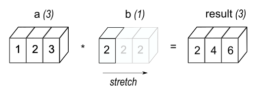
We could subtract a vector from a matrix
D - np.array([1,2,3])
Add a vector to a matrix
D + np.array([1,2,3])
We can use broadcasting for all sorts of applications. Use the mean function
and broadcasting to to mean center your data:
D-D.mean(axis=0)
or linalg.norm and broadcasting to scale your data so that each value is
between 0 and 1
D/np.linalg.norm(D)
... while I don't have a great reason why you would do this, it illustrates a useful function, write some code to mean center along the rows. Check out docs for mean and transpose for some help.
(D.transpose()-D.mean(axis=1)).transpose()
For one more exercise, let's compute the estimated variance for X0 (build up to that mess)
np.sum((X0-X0.mean())**2) / (X0.size-1)
0.1324763690893323
but, as you would expect, we could have just used numpy to begin with:
np.var((X0)
0.10598109527146585
... they are different?!! Do have an error? I double checked my code many times, what is going on here? Let's check the docs for np.var and there is this ddof optional argument. Ah, I see the problem "By default ddof is zero". The formula that we used in class was an unbiased estimate of the variance. So let's make sure we are using the right form:
np.var(X0, ddof=1)
0.1324763690893323
Bam! And to confirm our suspicions about the API and the ddof, what if we used the biased estimator of the variance:
np.sum((X0-X0.mean())**2) / (X0.size)
0.10598109527146585
that matches
np.var((X0)
0.10598109527146585
To quote Josh Starmer Double Bam!
So the takeaway here is libraries are great, but make sure to check the docs or you can end up with some pretty unexpected results.
Sometimes, it is just easier though to work on something on the web. So let's check out google collab. Go to https://colab.research.google.com/ and create a new notebook.
Let's try some of what we did before but this notebook:
def mean(X):
    acc = 0
    for xi in X:
        acc += xi
    return acc / len(X)


X = [8, 7, 9, 1, 5]
mean(X)
Okay, so that was way easier. And in fact, for some major libraries, we don't even need add dependencies:
import numpy as np
X = np.array([8, 7, 9, 1, 5])
x_hat =  X.sum() / X.size
And what is even better, we can "weave" together text and code.
For example I can put in text:
In the text, I can write markdown and then it is nicely rendered

For example, here is my list of things I need to do this afternoon

- eat a sandwitch
- teach data mining
- meet about yardstick
- drive home
- study the teachings of Topo Barktreuse
But where it really shines is when combing text and code. So we can have some text to provide context and then use the code to explain what is going on.
Prof Barktreuse collected data today about the snow levels the base of
Levrich canyon.  We can sumarize her findings as:
and then add a code block
import numpy as np
sample_snow_depts = np.array((3, 7, 2, 4, 5, 6, 5, 5, 5))
print(f"mean sample snow depth is {sample_snow_depts.mean()}")
and a text block
She wanted to understand how much variabliltiy there was in the show around
the base of the canyon so we can give an estimate the variance
and another code block
print(f"the variance is {sample_snow_depts.var(ddof=1)}")
and provide even more context
Note that when we called the variance function, we used the `ddof` argument,
setting this to 1 makes this an unbiased estimator of the variance.  For why
that is the case, see [Why dividing by N underestimates the
variance](https://www.youtube.com/watch?v=sHRBg6BhKjI)
This style of programming is not something that Google invented. And contrary to what you may have learned in from somebody that loves R, it is not something created by Hadley Wickham. What we were doing was using a programming paradigm created by Donald Knuth in the mid 1980's called Literate Programming. It has a ton of great uses (especially in data science) but maybe most immediately, it can be super useful when writing up your homework!
In fact, the tool you are using on collab, is just a web version of what is called a jupyter notebook There are lots of things that jupyter is useful for, but for the time being, we will just work with the notebooks. We can use conda to set up a jupyter notebook server locally by running the following:
conda install jupyter
and starting the notebook server locally (and show how we can do the same thing as on collab with a slightly different interface.) For the time being either is fine to use, whichever you are more comfortable with. I use both depending on which is easer for the thing I am trying to do.
A few other notes. These environments can become very complex in complex
projects, so it is often a good idea to capture your environment and keep it in
version control. Most often people keep it in a file called environment.yml.
We can export the environment with the following command:
conda env export --file environment.yml
This produces a file called environment.yml take a look at it. Note that
there is a line prefix in there. To my knowledge, it doesn't really get used
anywhere but if you for are hesitant about giving out information about your
file system, you can always delete that line.
So, I clam we can just blow way the old environment and then remake it, so let's give it a try:
conda activate base
conda env remove -n csci347
conda env list
and so it is gone. Let's remake it:
conda env create -f environment.yml
and to make sure, let's activate the csci347 environment
conda activate csci347
and just start a python shell and make sure that we can import numpy
import numpy as np
np.random.random((3,2))
Great! The carpentries is working on a really good tutorial for working with environments in conda. You can see it as it evolves at the Carpentries Incubaror.
So far, we have investigated how to use numpy as a useful library for implementing our primitive, but, often we are not given data as a matrix, but we have to do some work to get it to that format. Perhaps a format that is closer to what we will see in practice is data in a csv.
For example, consider the first few lines of data about the titanic from the pandas documentation
PassengerId,Survived,Pclass,Name,Sex,Age,SibSp,Parch,Ticket,Fare,Cabin,Embarked
1,0,3,"Braund, Mr. Owen Harris",male,22,1,0,A/5 21171,7.25,,S
2,1,1,"Cumings, Mrs. John Bradley (Florence Briggs Thayer)",female,38,1,0,PC 17599,71.2833,C85,C
3,1,3,"Heikkinen, Miss. Laina",female,26,0,0,STON/O2. 3101282,7.925,,S
4,1,1,"Futrelle, Mrs. Jacques Heath (Lily May Peel)",female,35,1,0,113803,53.1,C123,S
5,0,3,"Allen, Mr. William Henry",male,35,0,0,373450,8.05,,S
Aside from the non-numeric, which will will see how to encode in a bit, each column has meaningful names. When we are working with this data, wouldn't it be nice to refer to the fields by name instead of number. (For example, column "Survived" instead of column 1?). Pandas is an excellent library for working with tabular data. Let's try out a few examples. First, lets grab and load that titanic dataset. From your notebook
!curl https://raw.githubusercontent.com/pandas-dev/pandas/main/doc/data/titanic.csv --output titanic.csv
Aside: You could also run the command without the '!' from the terminal or download it from your browser. Download it in the notebook arguably the best option because it documents the location from where you fetched the data and helps to make the process you arrived at the final result reproducible. We will likely talk about reproducible research though out the semester.
We can peak at the data with the following command
!head titanic.csv
Okay, now let's install pandas and load this data in! From the command line, install pandas (make sure that you are working in the csci347 environment)
conda install pandas
Great! Let's hop back to our notebook. Import pandas and load the titanic data and look at the first few lines:
import pandas as pd
D = pd.read_csv("./titanic.csv")
D.head()
Look at how nice that data looks! So professional! All joking aside... you didn't really need to go though all those steps of downloading the data with curl and whatnot to get the data. I wanted to show you that so that you know how to get any data over an http connection. In reality, the following would work to load the data directly from github
D = pd.read_csv("https://raw.githubusercontent.com/pandas-dev/pandas/main/doc/data/titanic.csv")
Probably, the first thing we will want to do with pandas is get subsets of the data. For example, let's say we wanted to get a single column of data such as the passenger names. We can acccess this data similar to how we would data in a dictionary.
D["PassengerId"]
Note that while we only got one column, we have two columns of data. The first column is the row number of the data, the second column is the passenger's name. We can use the row numbers to access specific rows. For example to get the 3rd row.
D["Name"][3]
but, we will often want to get multiple columns, For example, imagine we wanted to get Name, Age, and if the passenger survived. We can get multiple columns with a standard python list:
D[["Name", "Age", "Survived"]]
For those interested in the details of python. The inner most list ["Name", "Age", "Survived"] is just a regular old python list and the outer D[...]
uses the python __getitem__ magic method on the pandas dataframe object.
One thing that we will often want to do when working with tables is select specific rows. random rant from here on out, we will use tables and dataframes interchangeably. While I personally don't care which you call it, most in the data science community would call them data frames and we want to be cool like them. back to our regularly scheduled jib-a-jaba
So, let's say you wanted to grab only the passengers that are over 20 years old. First, lets check out something super cool.
D["Age"] > 20
That "series" of booleans is of length number of rows. For any row in which the age was greater than 20, we will have a true, else we will have a false. So that is pretty nice, but it gets better. If have a series of trues and falses that is the same length as a data frame, we can get any row in which the value is true as.
D[ D["Age"] > 25 ]
This is probably one of the coolest and most helpful ideas that you can learn for easily getting subsets of data from a dataframe. And it doesn't stop there, you can create some pretty complex query criterion. In fact, for those that know SQL, many of the major relational algebra operations are implemented in the pandas api See Comparison with SQL for more.
One other thing to note, sometimes, you just want a few entries of the data for playing around, you can use
D.head()
to get the first 5 entries or specify the number that you want with
D.head(n=15)
Similarly you can get the last few lines with D.tail().
Note that sometimes, you may just want to make a data frame and not have a file to load in. In such a case, we can easily make one with the following code that builds a data frame of colors. (note that we mix strings and numbers)
df = pd.DataFrame([
    ['red', 255, 0, 0],
    ['blue', 0, 0, 255],
    ['green', 0, 255, 0],
    ['purple', 127, 0, 255],
])
df.columns=['name', 'R', 'G', 'B']
- some good data sets for trying things out
- representing categorical variables
- data visualisation