Stream Fusion and Merging
Platform for Situated Intelligence provides a set of stream operators and interpolators that allow the developer to easily implement a variety of stream fusion, merging and synchronization operations. This document describes these mechanisms.
Note: Prior to reading this document, we strongly recommend that you familiarize yourself with the core concepts of the \psi framework, by reading the Brief Introduction tutorial. The concepts of streams and originating times are a prerequisite for the documentation below.
The document is structured as follows:
- Fusion versus Merging - introduces the basic concepts of stream fusion and merging and the difference between the two.
- Stream Fusion: Interpolators - describes interpolators, which are a core construct enabling stream fusion and synchronization.
- Stream Fusion: Components and Operators - describes existing components and stream operators for performing stream fusion.
- Stream Merging - describes existing components and stream operators for performing stream merging.
Suppose that we have two streams s1 and s2 that produce messages, as illustrated in the figure below. These might be streams of the same type, or of different types (say audio and video), each with their own (not necessarily equal or even constant) cadence.

A fusion operation takes two such streams as input (as we shall see later, this can be generalized to more than two), and produces a single output stream. Each output message is constructed by fusing a pair of messages from the input streams. In general, the type of the output messages might be different than the type of the inputs: each output get generated by applying a function to a pair of inputs. Since the messages arrive on the two input streams on their own timing, the fundamental problem the fusion component has to resolve is therefore how to pair the messages on the two input streams. We discuss this question, and fusion stream operators (Fuse and Join) in sections 2 and 3 below.
In contrast, a merging operation combines streams of the same type. If in fusion the output messages are generally of a different type, a merging operation simply outputs the incoming messages one by one on the resulting stream, as illustrated by the figure below.

Evidently, in this case the input and output streams are of the same type. As with fusion, since the incoming messages arrive with different latencies on the input streams, various options are available in terms of ordering these messages on the output stream. We discuss this, and the corresponding stream merging operators (Merge and Zip) in section 4 below.
As we have seen above, a central question that arises in a fusion operation is how to pair the input messages. Certain applications might have different requirements around how this pairing should be done. For instance in one case we might want to pair messages from s1 with the closest message in originating time from s2 (this pairing is illustrated in the figure above); in another case we might want to pair it with the last message available on s2, and so forth. In \psi, this pairing problem is resolved via interpolators, which we describe below.
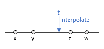
An interpolator specifies how a generate a new message at a given interpolation time, from a stream of messages. The \psi framework provides a number of such interpolators, and new ones can also be created. For instance, one of the simplest interpolators, called Reproducible.Nearest, generates as an interpolation result the nearest message to the interpolation time. If we use this interpolator over the messages shown in the figure below to interpolate at the time shown as t, the interpolation result would be message z. The Reproducible.Nearest interpolator simply selects a message from the existing stream, but in general an interpolator can create new messages (e.g., a linear interpolator between two points).
Fusion components (such as Fuse and Join discussed later) fuse data from a primary stream with a secondary stream by applying a specified interpolator: for every message received on the primary stream, the interpolator is called over the secondary stream to produce a message that the primary message should be paired with. For example, the pairing that results when fusing s1 as a primary stream with s2 as a secondary stream, using the Reproducible.Nearest interpolator is illustrated below:

Notice that for each message on the primary stream one (or possibly zero) messages may be produced on the output, fused stream. At the same time, a message on the secondary stream may be used multiple times in the fusion process. For instance, in the example above, z was the nearest message on the secondary stream for both c and d.
By default, the Reproducible.Nearest interpolator we have introduced above looks for the nearest message on the entire secondary stream. The interpolator can be customized however with an optional parameter that specifies a time window or time tolerace, relative to the interpolation time, that should be considered when looking for the nearest match.
Relative time windows are represented via the RelativeTimeInterval class, which provides a number of constructors and static methods that enable creating a variety of relative time windows, shown in the table below.
| Expression | Relative time window |
|---|---|
RelativeTimeInterval.Infinite |
(-∞, +∞) |
RelativeTimeInterval.Empty |
(0, 0) |
RelativeTimeInterval.Zero |
[0, 0] |
RelativeTimeInterval.Past() |
(-∞, 0] |
RelativeTimeInterval.Future() |
[0, +∞) |
new RelativeTimeInterval(TimeSpan.FromSeconds(-2), TimeSpan.FromSecond(3)) |
[-2, 3] |
new RelativeTimeInterval(TimeSpan.FromSeconds(-5), true, TimeSpan.Zero, false) |
[-5, 0) |
For instance, if we wish to select the nearest message before time t, we can construct a relative time window that from minus infinity (e.g. infinite past) to zero (e.g., present moment) via RelativeTimeInterval.Past(). Interpolating at time t with a Reproducible.Nearest(RelativeTimeInterval.Past()) in the figure below selects message y, as this is the closest message to time t, when looking in the past.

If we use a Reproducible.Nearest(RelativeTimeInterval.Past()) interpolator to fuse the streams s1 and s2, the pairing that results is illustrated below -- each message on the primary stream s1 is paired with the previous message on s2:

Instead of relative time intervals, an optional time tolerance parameter can also be specified as a TimeSpan, and is automatically converted into a symmetric relative time interval, for instance:
Reproducible.Nearest(TimeSpan.FromSeconds(1)))
is equivalent to:
Reproducible.Nearest(new RelativeTimeInterval(TimeSpan.FromSeconds(-1), TimeSpan.FromSeconds(1)))
The list of interpolators extends well beyond the Reproducible.Nearest interpolator discussed above. Interpolators are implemented as classes that derive from Interpolator<TIn, TResult> and most of them are directly accessible via static factory methods on the Reproducible and Available classes, as shown in the table below:
| Interpolator | Description |
|---|---|
| Reproducible Interpolators | |
Reproducible.Exact() |
Selects the message with the same originating time as the interpolation time. |
Reproducible.Nearest<T>(...) |
Selects the nearest message (within a relative time interval or time tolerance) to the interpolation time. |
Reproducible.First<T>(...) |
Selects the first message (within a relative time interval or time tolerance) to the interpolation time. |
Reproducible.Last<T>(...) |
Selects the last message (within a relative time interval or time tolerance) to the interpolation time. |
Reproducible.Linear(...) |
Produces an interpolation result over a stream of doubles by linear interpolation between the messages before and after the interpolation time. |
AdjacentValuesInterpolator(...) |
Produces an interpolation result over a generic stream by applying a user-specified function to the messages adjacent (before and after) to the interpolation time. (The linear interpolator above is based on this adjacent values interpolator.) |
| Greedy Interpolators | |
Available.Exact() |
Selects from the messages already available on the interpolation stream the message with the same originating time as the interpolation time. |
Available.Nearest<T>(...) |
Selects from the messages already available on the interpolation stream the nearest message (within a relative time interval or time tolerance) to the interpolation time. |
Available.First<T>(...) |
Selects from the messages already available on the interpolation stream the first message (within a relative time interval or time tolerance) to the interpolation time. |
Available.Last<T>(...) |
Selects from the messages already available on the interpolation stream the last message (within a relative time interval or time tolerance) to the interpolation time. |
The Nearest, First and Last interpolators from the table above also come in an OrDefault flavor, e.g. NearestOrDefault, FirstOrDefault, LastOrDefault (not shown in the table for compactness). When a Nearest, First or Last interpolator does not find a corresponding match for a primary message (e.g. there is no matching secondary message in the specified interpolation window, etc.), no message will be produced on the output stream for that primary message. With the OrDefault version a default secondary stream value will be produced instead in this case. For instance, the Figure below shows the results over our example streams s1 and s2, when using Reproducible.Nearest(RelativeTimeInterval.Past()) versus Reproducible.NearestOrDefault(RelativeTimeInterval.Past(), '0'). The default value to be used can be specified by the developer, or it itself defaults to default(T).
As the table above indicates, the interpolators in the \psi framework are divided into two broad categories: called reproducible interpolators and greedy interpolators. The important difference between these two classes is that the reproducible interpolators will always generate the same provably-correct result, regardless of the arrival time of the messages, whereas the greedy ones do not provide this guarantee. This is a very important point, as it significantly changes the behavior of data fusion -- we discuss it in depth below.
To explain the difference between reproducible and greedy interpolators, let's look back at a concrete example involving the streams s1 and s2 we have introduced earlier. In the figures above we have illustrated the messages on a horizontal time axis, at the position corresponding to their originating times. Note however that these messages might arrive with arbitrary latencies. And, while they will always appear in the order of the originating times on an individual stream, the arrival order might be different across streams because of the delays with which the message arrive.
Consider for instance the two examples below.

Each shows the same messages with the same originating times, but appearing in different orders. In example 1, a appears (1st), then x (2nd), then b (3rd), y (4th), c (5th), z (6th), d (7th), w (8th) and finally e (9th). In this case the messages appear across streams actually in increasing originating time order. This however is most often not the case, as the example on the right-hand side shows. In this example , x appears (1st), then a (2nd), b (3rd), and c (4th) appear, followed by y (5th), then d (6th), then z (7th) and w (8th), and finally e (9th).
The reproducible interpolators will produce the same result, regardless of the order in which the messages appear on the two streams. In contrast, let's look the other, greedy version of the "nearest" interpolator, called Available.Nearest. This interpolator also selects the message nearest in originating time to the primary message, but it does so by looking only at the messages that are currently available on the secondary stream when the interpolator is first queried (e.g. when the primary message arrives) -- hence the name greedy. In contrast, the Reproducible.Nearest interpolator will potentially "wait" for new messages until it accumulates enough evidence that it has the correct answer, no matter what other messages might arrive on the secondary stream.
As a result, performing fusion via the Reproducible.Nearest interpolator will produce the same set of pairs for both examples above: (a,x), (b,y), (c,z), (d,z), (e,w).

In contrast, the results produced by the Available.Nearest operator depend not just on the originating times, but also on the order of arrival across streams that is induced by the latency of the messages. In example 1, the Available.Nearest interpolator will produce: (b,x), (c,y), (d,z), (e,w). Note that in this example no output is generated corresponding to the primary stream message a, as no secondary message is already available at the time a arrives. In example 2, the output of Available.Nearest will again be different: (a,x), (b,x), (c,x), (d,x), and (e,w).

There is a fundamental tradeoff between the reproducible and greedy interpolators: reproducible interpolators will produce the correct results in terms of originating time regardless of the latency at which the messages arrive, but they do so at the potential cost of introducing more latency. This is the case because the reproducible interpolators have to see enough messages on the secondary stream to guarantee that the result they output will never change, regardless of what else might appear in the future on the secondary stream.
For instance, in the situated from example 2 we have shown above (see again below), at the time message c arrives on the primary, the only message available on the secondary stream is x, and this is the nearest message at this point in time. However, at this point in time the interpolator "knows" that other messages might arrive on the secondary stream that might be even closer in originating time, so it does not create an output. The interpolator waits in essence until it sees a message z in this case. Once z appears, it is clear that no future messages arriving on the secondary stream will change the answer, and an output is created. Note however that in the meantime other messages have arrived (d and y), including even messages on the primary stream (d) -- the fusion components are queuing these messages and will process them later on. In effect, in the case above, to generate an interpolation result for c we have to wait until z arrives. As a consequence the cadence and latency of the secondary stream dictates the latency of the interpolation result and fusion process.
In contrast the greedy, Available.* version of the interpolators produce the result right away, as the primary message arrives, but they only take into account what is present at that moment on the secondary stream, and as such might generate less precise, and generally non-reproducible results. They however do not incur the latency of the messages on the secondary stream.
Having introduced the various types of interpolators above we now finally turn attention back to data fusion. Data fusion in \psi can be accomplished via one of two data fusion components and corresponding sets of stream operators: Fuse and Join. Both components use interpolators to determine how messages on a secondary and primary streams are paired and used together to generate a fused result.
Fuse is the most general data fusion component/operator, and can use any type of interpolator. In contrast, Join is a component that derives off of Fuse, and only allows for using reproducible interpolators. The distinction was introduced as a way to syntatically highlight in the code written when a reproducible fusion is performed versus not, i.e. Join means reproducible.
Other than this distinction, the usage for these two operators is very similar, and is illustrated below with a few examples, based on Join.
The basic syntax for joining two streams is:
var joined = primary.Join(secondary);In this case, primary and secondary are the primary and secondary streams respectively. Join is a stream operator that applies to the primary stream, and takes as a first parameter the secondary stream. If no interpolator is specified, as in the example above, Join assumes by default the Reproducible.Exact interpolator -- this requires that the messages in the secondary stream align exactly in originating time with the primary stream messages. However, an interpolator can be specified by the developer, either directly:
var joined = primary.Join(secondary, Reproducible.Nearest(RelativeTimeInterval.Past()));or by providing a relative time interval or a time tolerance, in which case a Reproducible.Nearest interpolator with that corresponding time window is assumed:
var joined = primary.Join(secondary, RelativeTimeInterval.Past());By default, in the examples aboved the joined stream will be a stream of tuples of elements (p, s), where p is an element from the primary stream and s is an element from the secondary stream. Alternatively, Join and Fuse accept as an optional parameter a fusion-function that maps the paired values to a different output type. For instance, if primary and secondary are two integer streams:
var joined = primary.Join(secondary, RelativeTimeInterval.Past(), (p, s) => p + s);will construct a joined stream of integers, where each fused integer output is the sum of the two inputs.
Finally, Join and Fuse also accept two additional parameters named primaryDeliveryPolicy and secondaryDeliveryPolicy which control the delivery policies on the primary and secondary stream connections. By default, the pipeline-level delivery policy will be used.
When sequentially fusing multiple streams without explicitly specifying a fusion-function, the end result would naturally be a tuple of tuples. For example, a.Join(b).Join(c).Join(d) would produce a tuple of the form (((a, b), c), d). This was deemed unwieldy, and to remedy it, a number of versions of Join(...) and Fuse(...) operators are available for streams of the type IProducer<ValueTuple<...>> which produce flattened tuples up to an arity of 7. This way a.Join(b) produces (a, b) but then .Join(c) produces (a, b, c) and further .Join(d) produces (a, b, c, d). We refer to this as tuple-flattening.
A stream of scalar (or otherwise non-tuple) values joined with a stream of ValueTuple<...> also produces a flattened tuple stream. That is, aside from a.Join(b).Join(c).Join(d) producing (a, b, c, d) as above, the following does as well:
var cd = c.Join(d); // (c, d)
var bcd = b.Join(cd); // (b, c, d)
var abcd = a.Join(bcd); // (a, b, c, d)Another version of the Join and Fuse operators enable vector fusion. Vector fusion operates with a single primary stream (IProducer<TPrimary>), as usual, but with a sequence of secondary streams. That is, an enumeration of secondary streams (IEnumerable<IProducer<TSecondary>>) can be provided. All the secondary streams must have the same type. A fusion-function mapping from a pair of TPrimary and TSecondary[] to a new, fused output type must be provided.
Based on this vector-fusion version, Join and Fuse overloads are also available that simply take as input a single array of streams of a given type, and fuse them in a vector. For example, assuming streams is an enumeration of streams, i.e. IEnumerable<IProducer<T>>:
var vectorStream = Operators.Join(streams, Reproducible.Nearest());the resulting vectorStream will be a stream of vectors of type T, i.e. IProducer<T[]>. This is implemented by using the first stream in the streams enumeration as a primary, and all the other streams as secondary streams in a vector-fusion operation.
Apart from Fuse and Join, the Pair operator can also be used to perform data fusion, but mostly exists for historical reasons and might be deprecated in the future.
Pair behaves in essence like a Fuse with a greedy Available.LastOrDefault() interpolator: as soon as primary message is received, it will pair it with the last received secondary message, and output the corresponding tuple. Like with Fuse and Join, overloads are available to perform tuple flattening, and also to allow specifying a fusion function and primary and secondary delivery policies.
Having discussed stream fusion, we now turn attention to merging. Recall that in a merging operation, the inputs and outputs have the same type and the output stream will essentially contain the messages from all input streams.
There are two operators that enable stream merging in the \psi framework: Merge and Zip.
The Zip operator merges two or more streams, based on the originating time of the incoming messages, and regardless of the latencies of arrival. Zip is therefore reproducible. As we have seen in the example 2 above, messages do not necessarily arrive in originating time order across streams. For instance, below the x message is received first, even though its originating time is larger than that for message a. However, Zip knows that it cannot immediately post x and caches it until the appropriate time to post. The messages are posted by Zip in originating time order, as illustrated below.

Because Zip is reproducible, same tradeoff between latency and reproducibility we have discussed with Join and reproducible interpolators arises here: before posting a specific input message, the operator needs to receive enough messages on its input streams to guarantee that no other message could appear with on originating time smaller than the one for the message to be posted. For instance, in the example above, Zip only posts x after it has received x, a and b (only once b is seen we know for sure that no other message will arrive on the first stream with an originating time smaller than that of x).
Finally, we note that the Zip operator produces messages of type T[], rather than just T (where T is the input type). In general, the array contains a single element with the input message. However, if messages arrive on the two (or more) input streams with the exact same originating time, they will be collated into an array and posted together, at that originating time (recall that in \psi we cannot post multiple messages with the same originating time on a stream).
In constrast to Zip, the Merge operator posts incoming messages as they arrive, and therefore incurs no latency. However, to handle the fact that messages on the incoming streams might arrive out of originating-time order (across streams), the Merge operator posts on the output a message that contains as the payload, not just the input data, but rather the entire input message. Merge takes therefore as input a stream of type T (i.e. IProducer<T>), and produces as input a stream of type Message<T> (i.e. IProducer<Message<T>>). The originating time for each output message (of message) is the time of the input's arrival at Merge, rather than the originating time of the input. The timing of the posted output messages no longer corresponds to the originating times of the incoming messages. The figure below illustrates the Merge operator.

Since the output stream contains as payload the entire input message though, the originating time of the inputs is still available for downstream components to use. For example the payload M[x] is a Message<T>, which contains the envelope for the message x. A downstream component could in principle listen to the output of merge, cache things the incoming messages, and reorder them in an application-specific way.